Load the R package we will use.

library(tidyverse)
library(moderndive)

Quiz questions

-Replace all the instances of ‘SEE QUIZ’. These are inputs from your moodle quiz.

-Replace all the instances of ‘???’. These are answers on your moodle quiz.

-Run all the individual code chunks to make sure the answers in this file correspond with your quiz answers

-After you check all your code chunks run then you can knit it. It won’t knit until the ??? are replaced

-The quiz assumes that you have watched the videos and worked through the examples in Chapter 7 of ModernDive

Question:

7.2.4 in Modern Dive with different sample sizes and repetitions

-Make sure you have installed and loaded the tidyverse and the moderndive packages

-Fill in the blanks

-Put the command you use in the Rchunks in your Rmd file for this quiz.

Modify the code for comparing different sample sizes from the virtual bowl

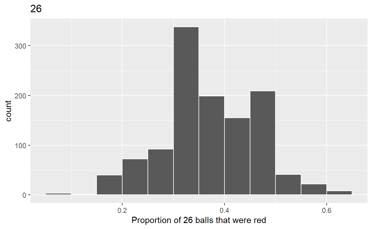
Segment 1: sample size = 26

1.a)Take 1180 samples of size of 26 instead of 1000 replicates of size 25 from the bowl dataset. Assign the output to virtual_samples_26

virtual_samples_26 <- bowl %>% 
  rep_sample_n(size = 26, reps = 1180)

1.b)Compute resulting 1180 replicates of proportion red

-start with virtual_samples_26 THEN

-group_by replicate THEN

-create variable red equal to the sum of all the red balls

-create variable prop_red equal to variable red / 26

-Assign the output to virtual_prop_red_26

virtual_prop_red_26 <- virtual_samples_26 %>% 
  group_by(replicate) %>% 
  summarize(red = sum(color == "red")) %>% 
  mutate(prop_red = red / 26)

1.c)Plot distribution of virtual_prop_red_26 via a histogram use labs to

-label x axis = “Proportion of 26 balls that were red”

-create title = “26”

ggplot(virtual_prop_red_26, aes(x = prop_red)) + 
  geom_histogram (binwidth = 0.05, boundary = 0.4, color = "white") +
  labs(x = "Proportion of 26 balls that were red", title = "26")

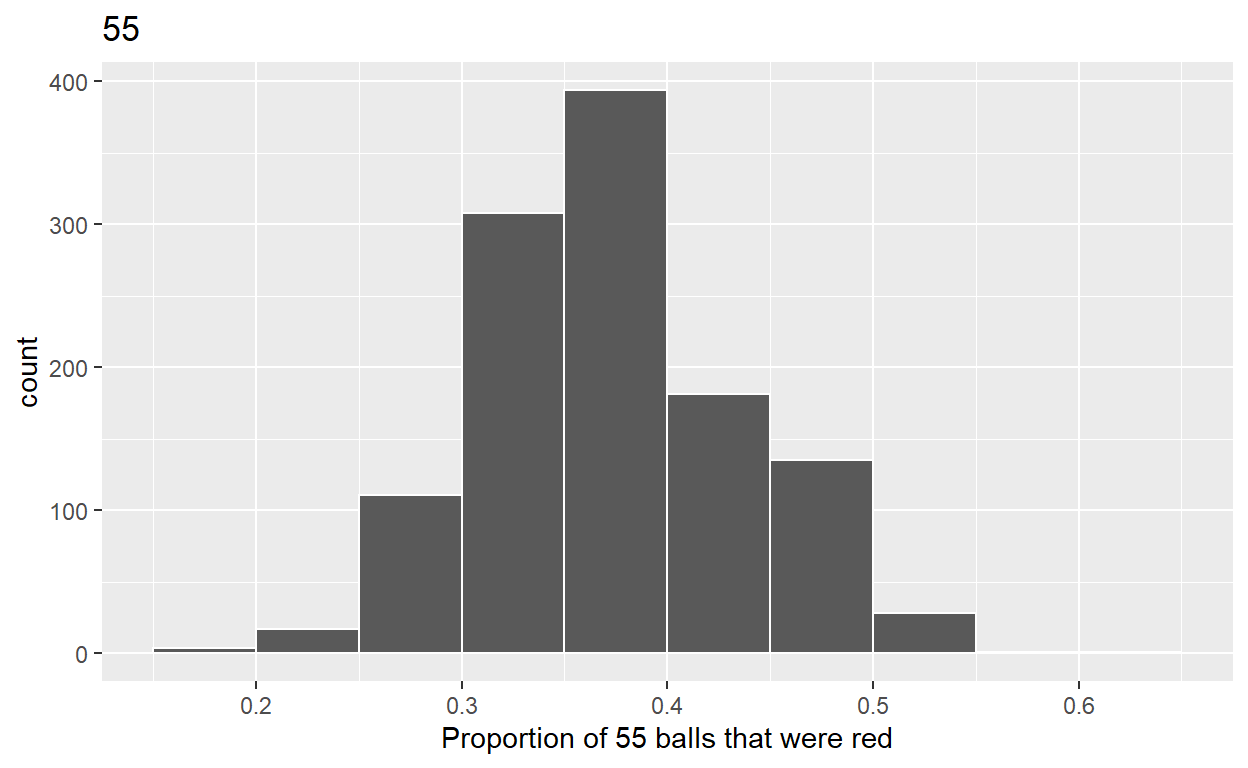
Segment 2: sample size = 55

2.a)Take 1180 samples of size of 55 instead of 1000 replicates of size 50. Assign the output to virtual_samples_55

virtual_samples_55 <- bowl %>% 
  rep_sample_n(size = 55, reps = 1180)

2.b)Compute resulting 1180 replicates of proportion red

-start with virtual_samples_55 THEN

-group_by replicate THEN

-create variable red equal to the sum of all the red balls

-create variable prop_red equal to variable red / 55

-Assign the output to virtual_prop_red_55

virtual_prop_red_55 <- virtual_samples_55 %>% 
  group_by(replicate) %>% 
  summarize(red = sum(color == "red")) %>% 
  mutate(prop_red = red / 55)

2.c)Plot distribution of virtual_prop_red_55 via a histogram use labs to

-label x axis = “Proportion of 55 balls that were red”

-create title = “55”

ggplot(virtual_prop_red_55, aes(x = prop_red)) +
  geom_histogram(binwidth = 0.05, boundary = 0.4, color = "white") +
  labs(x = "Proportion of 55 balls that were red", title = "55")

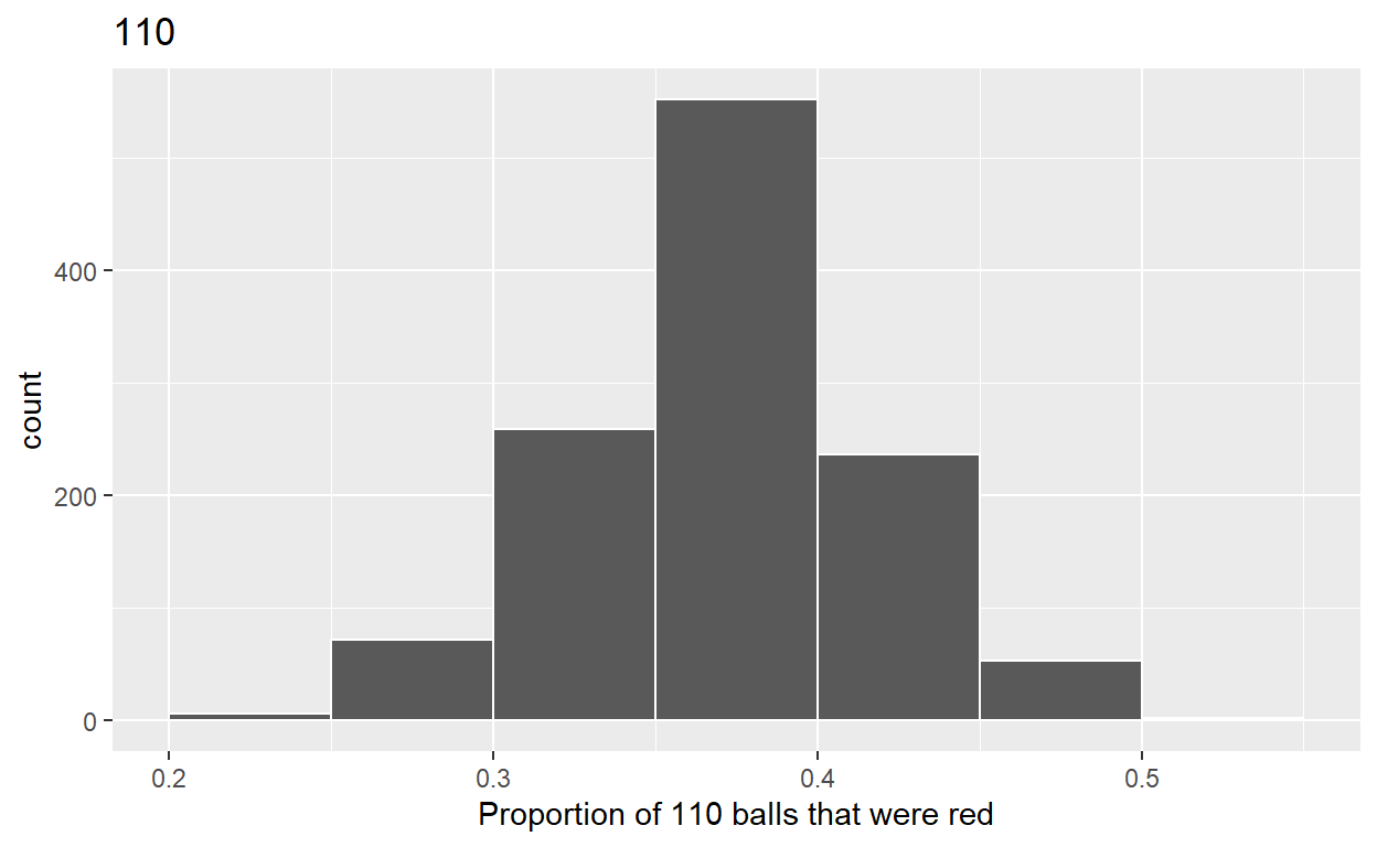
Segment 3: sample size = 110

3.a)Take 1180 samples of size of 110 instead of 1000 replicates of size 50. Assign the output to virtual_samples_110

virtual_samples_110  <- bowl %>% 
  rep_sample_n(size = 110, reps = 1180)

3.b)Compute resulting 1180 replicates of proportion red

-start with virtual_samples_110 THEN

-group_by replicate THEN

-create variable red equal to the sum of all the red balls

-create variable prop_red equal to variable red / 110

-Assign the output to virtual_prop_red_110

virtual_prop_red_110 <- virtual_samples_110 %>% 
  group_by(replicate) %>% 
  summarize(red = sum(color == "red")) %>% 
  mutate(prop_red = red / 110)

3.c)Plot distribution of virtual_prop_red_110 via a histogram use labs to

-label x axis = “Proportion of 110 balls that were red”

-create title = “110”

ggplot(virtual_prop_red_110, aes(x = prop_red)) + 
  geom_histogram(binwidth = 0.05, boundary = 0.4, color = "white") +
  labs(x = "Proportion of 110 balls that were red", title = "110")

Calculate the standard deviations for your three sets of 1180 values of prop_red using the standard deviation

n = 26

virtual_prop_red_26 %>% 
  summarize(sd = sd(prop_red))

# A tibble: 1 x 1
      sd
   <dbl>
1 0.0930

n = 55

virtual_prop_red_55 %>% 
  summarize(sd = sd(prop_red))

# A tibble: 1 x 1
      sd
   <dbl>
1 0.0634

n = 110

virtual_prop_red_110 %>% 
  summarize(sd = sd(prop_red))

# A tibble: 1 x 1
      sd
   <dbl>
1 0.0451

The distribution with sample size, n = 110, has the smallest standard deviation (spread) around the estimated proportion of red balls.

Sampling

Question: