- Packages I will use to read in and plot the data
- Read the data in from part 1
Interactive graph
- Start with the data
- Graph_by symptom so there will be a “bar” for each symptom
- Use mutate to round NAA so only 2 digits will be displayed when you hover over it
- Use e_charts to create an e_charts object with Symptom on the x-axis
- Use e_bar to build that contain NAA by symptoms. The depth of each bar represents the amount of emissions for each symptom.
- use e_tooltip to add a tooltip that will display based on the axis value
- use e_title to add a tittle, subtitle, and link to subtitle
- use e_theme to change the theme to roma
Depression_symptoms_not_shown %>%
  mutate(NAA = round(NAA, 2)) %>%
  arrange(NAA) %>%
  e_charts(x = Symptoms) %>%
  e_bar(serie = NAA, legend = FALSE) %>%
  e_flip_coords() %>%
  e_tooltip(trigger = "axis") %>%
  e_title(text = "Depression Symptoms not shown",
          subtext = "(in 2014) Source; Our World in Data",
          sublink = "https://ourworldindata.org/what-is-depression",
          left = "center") %>%
  e_theme("roma")
static graph
- start with data
- use ggplot to create a new ggplot object. Use aes to indicate that symptoms will be mapped to the x-axis; NAA will be mapped to the y-axis; symptoms will be the fill variable
- geom_col will display NAA
- theme_classic sets the theme
- theme(legend.position = “bottom”) puts the legend at the bottom of the plot
- labs sets the y-axis label, fill = NULL indicates that the fill variable will not have the labelled Region
Depression_symptoms_not_shown %>%
  ggplot(aes(x = Symptoms, y = NAA)) +
  geom_col() +
  coord_flip() +
  theme_classic() +
  theme(legend.position = "bottom")
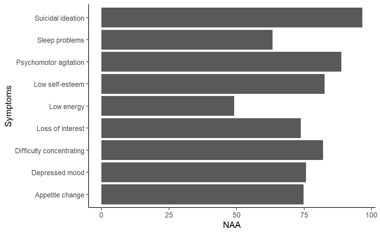
These plots show the the rate of which symptom was not shown at all.